Category: Machine Learning

In this one, I want to talk about the output of data. How we frame the output of an algorithm is as delicate as the original choice of algorithm itself. The informal cycle I have been working with has been data sourcing and preparation, followed by processing (applying statistical methods and machine learning algorithms), and then presenting that in a form that people can understand.

In each of these procedural points, decisions have to be made.

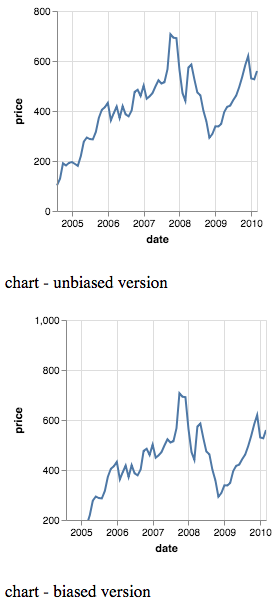
Take a gander at the following two charts:

They look different. But they also look the same. What accounts for this? In the second chart, a great deal of empty space up top evokes some kind of downward, negative pressure. Assuming that the viewer is a native user of a language that reads left-to-right, top-to-bottom, one might be inclined to say that the first graph shows good performance, and the second indicates worse performance.

On closer examination, however, there is no actual difference in the graph. The differences are in the y-axis. In the second chart, the y-axis begins at 200 (rather than 0), and goes all the way up to 1000. The peak, just before 2008, remains just over 700 in both graphs. Both charts use and represent the same data without any distortion. So the manipulation is at the framing-level.

Future installments will cover some sneakier ways to present data. The source code for this example can be found here on my github.

To see the entire Machine Learning Tutorial, go here.

Remember that boring data?

NAME	COUNTRY	OWN A CAR	LIKES ICE-CREAM
Eliza Santiago	Guatemala	Yes	No
Fred Winchester	Canada	No	Yes
Marvin Ngoma	Ghana	Yes	No
Xiong Mao	USA	Yes	???

This example may remind some of the battered adage that “correlation does not imply causality.” This cautionary statement is often the only thing people remember from their brief exposure to statistics. While it is certainly useful, it is not entirely the case.

Let’s remove the extraneous details such as the name and country, replacing them with a generic, indexed tag. After all, we aren’t really (at this point), interested in whether certain details such as the number of vowels in a name, or what part of the world we find a country, have any impact on car ownership or ice-cream preference. To take those into account would be to introduce overfitting, which is the phenomenon of having so much information in a model that it becomes burdensome to separate the data that has a causal effect from that which we ought to consider arbitrary.

To take it a step further, let’s generalize car ownership and ice-cream preference to “A” and “B.” We obtain something very similar to a truth table in deductive logic.

NAME	COUNTRY	A	B
n1	c1	A	NOT-B
n2	c2	NOT-A	B
n3	c3	A	NOT-B
n4	c4	A	???

One of the early promises of inductive and probabilistic models is that by putting data into a sophisticated enough machine, hidden rules will emerge. From this it can become really tempting to treat these hidden rules as having deductive weight, in the same way that statements such as “all birds have wings” and “all creatures with wings can fly” allow one to deduce “all winged creatures can fly.” But there are massive problems with this beyond mere arrogance. The biggest problem is that with data obtained in the wild may not have been generated from a deductive rule (if A then B). With my personal methodology, chaos typically reigns supreme.

One is a threshold problem. As I see it, what is the ideal threshold between underfitting (too little data to gleam any decent insight) and overfitting (too much data to get a reliable model that can provide accurate results in a reasonable amount of time)?

Consider this model:

Animal	Feathers?	Wings?	Can Fly?
Merlin	Yes	Yes	Yes
Kiwi	Yes	No	No
Dolphin	No	No	No
Vampire Bat	No	Yes	???
Penguin	Yes	Yes	???

Here, we give our inductive engine (i.e. a machine learning agent) a lot of details from which to issue decisions. We could assume that this engine is intelligent enough not to take “the animal’s name ends with –in” as a criteria, but that is a bold assumption. Sure, if we are doing supervised machine learning, then we should train our machine to answer whether a given animal can fly, based off of a combination of the most relevant information. But just how this machine agent knows what information is relevant and which should be considered a coincidence lays squarely on the humans training that machine.

In unsupervised models, we can’t make the assumption that machines won’t learn from superfluous details such as whether an animal’s name ends with –in or not. Adding the generic, indexed tags as animal names, similar to the tags in the second table of this lesson, can sidestep this and lessen the risk of overfitting.

Given the data on Merlins, Kiwis, Dolphins, Vampire Bats, and Penguins, what answer should we expect regarding bats’ and penguins’ ability to fly?

To see the entire Machine Learning Tutorial, go here.

Let’s start with the data.

Data just means “that which is given” in Latin. If I handed you a muffin, that’s data. But that’s not the data we’re going to think about. Data in this case typically means a bunch of information, and we need to extract that information from a source, put it into a format a machine can read, and then parse it in order to gleam something that isn’t immediately obvious from first examination.

What we’re given can be a picture, or a string of letters. The task of machine learning is to infer from what is given, those things that are not given. In some cases, humans will assist in a training role. That is, a person will be asked to identify what object(s) are in a picture (is it a fire hydrant? is it a car?) or what a sentence means. In other cases, there will be no training, and the machine will learn from just the data.

This concept translates fairly well over both visual and linguistic cases, but the linguistic case is a bit easier to start with.

So let’s consider some really boring data.

NAME	COUNTRY	OWN A CAR	LIKES ICE-CREAM
Eliza Santiago	Guatemala	Yes	No
Fred Winchester	Canada	No	Yes
Marvin Ngoma	Ghana	Yes	No
Xiong Mao	USA	Yes	???

We have some made-up people: Fred Winchester, Eliza Santiago, Marvin Ngoma, and Xiong Mao. And we have their phone numbers, the type of ice-cream they like, and if they drive a car. From this, we must ask part of the data we actually need and what is extraneous. Phone numbers are assigned in a largely arbitrary (but not necessarily random) fashion.

For the sake of reducing details (and thereby lessening the possibility of overfitting), we ought to either discard the phone number entirely, or at least reduce it to just the country code (say, +44 for the UK) and area code prefix. Let’s assume we had their name, their number, and the answer to at least one of the questions about their ice cream preferences and whether they drive.

So the easy question is, provided with this information, do we have sufficient data to know Xiong Mao’s ice cream preference?

The harder question is why this information is or is not sufficient. In subsequent installments of this tutorial I will go into the arguments for and against whether we can make a deductive claim off of incomplete information (this being one of the core premises and promises of machine learning).

To see the entire Machine Learning Tutorial, go here.

In this multi-part tutorial, I shall go over the basics of taking “live” human data and putting into a suitable format to feed into one’s machine learning platform of choice. This series will go from general to specific and offer insight on methodology before going into gathering data, putting this data into a machine-readable format, and then feeding this into machine learning platforms such as TensorFlow and Weka.

To start, I have to think of the data set in at least two lights.

One is theme-oriented: the data has to have a thematic character that is neither too broad as to capture spurious correlations, and not so narrow that it confirms the obvious. This is the story told by the data.

The other is feature-oriented. A good data set needs to have its raw data converted into a workable ontology — which is just a fancy word to refer to the objects and the landscape they inhabit. These are the nouns of story told by the data.

These are methodological, but reflect a deeper concern: doxology. What human belief do these reinforce? Will these reinforce a prevailing status quo, something people take as a given, or will the data be such that new insights can be gleamed? This goes beyond merely trying to avoid overfitting (when data is so finely grained that it has too many details and thereby has too much extraneous information to report to be of much use). This means making sure that if your data set is going to be free from racial bias, care has been taken to remove proxies for racial demographics, such as zip code.

Summary of results: which methodology/modality “wins?”

		Vanilla				Merged
Algorithm	Speed	CCI %	ROC AUC	RMSE	F-1	CCI %	ROC AUC	F-1	RMSE
ZeroR	Instant	37.9333	0.4990	0.4144	NULL	47.1000	0.4990	NULL	0.4536
OneR	Instant	43.0000	0.5420	0.5339	NULL	52.9833	0.5660	NULL	0.5599
NaiveBayes	Fast	63.8500	0.8160	0.3808	0.6410	63.9667	0.8000	0.6430	0.4374
IBK	Fast	56.5333	0.6910	0.4386	0.5230	59.5833	0.6510	0.5470	0.4972
RandomTree	Fast	59.5833	0.6800	0.4474	0.5920	62.7167	0.6700	0.6210	0.4954
SimpleLogistic	Moderate	73.6500	0.8850	0.3065	0.7320	73.6500	0.8730	0.7300	0.3502
DecisionTable	Slow	too slow for viable computation on consumer-grade hardware
MultilayerPerceptron	Slow
RandomForest	Slow
		Vanilla				Merged
Meta-Classifier	Speed	CCI %	ROC AUC	RMSE	F-1	CCI %	ROC AUC	F-1	RMSE
Stack (ZR, NB)	Moderate	37.9333	0.4990	0.4144	NULL	vacuous results, omitted
Stack (NB. RT)	Moderate	63.7000	0.8230	0.3795	0.6350	61.9833	0.6980	0.6130	0.4523
Vote (ZR, NB, RT)	Moderate	62.0833	0.8430	0.3414	0.6110	64.0500	0.8330	0.6260	0.3830
CostSensitive (ZR)	Instant	37.9333	0.4990	0.4144	NULL	36.6667	0.4990	NULL	0.4623
CostSensitive (OR)	Instant	42.7000	0.5400	0.5353	NULL	39.6167	0.5170	NULL	0.6345
CostSensitive (NB)	Fast	63.8500	0.8160	0.3808	0.6410	64.0833	0.8010	0.6450	0.4365
CostSensitive (IBK)	Fast	56.5333	0.6910	0.4386	0.5230	59.5833	0.6510	0.5470	0.4972
CostSensitive (RT)	Fast	59.5833	0.6800	0.4474	0.5920	63.3833	0.7050	0.6350	0.4728
CostSensitive (SL)	Moderate	73.6500	0.8850	0.3065	0.7320	74.7833	0.8780	0.7450	0.3478

My results are contained in a separate text file in lab journal format. Salient results consisted of:

Continue reading “Summary: Machine Learning on the Rosanne-ABC Firing Incident Dataset” →